Thoughts on Applying Research

I am concluding this blog differently than I anticipated. I have not completed reading all of the materials, and plan to do so, but as I graduate in two days I thought I should provide a conclusion of sorts.

Yesterday I was at the laundromat where I witnessed a discussion between a (clearly wealthy) customer and a laundry attendant. The customer was asking the attendant how much it would cost to have the staff wash her son’s bedsheets (I know, typical). The attendant told her it would be $8 but that she couldn’t guarantee it would be  completed by the end of the day. After considering her options, the customer decided she would simply do it herself. “I will tell you a secret,” said the attendant, “it will be cheaper if you do it yourself.” The customer replied “Oh, well that wasn’t…” and then mumbled something about saving time.

Most people wouldn’t think twice about this discussion but I found myself in many ways mentally translating for the two women. Poor people think differently, and having grown up relatively poor I understand this mindset. To the attendant, a $4 difference between washing your own laundry and paying for someone else to do it is meaningful. It means you would have $4 for lunch. To the customer, $4 was menial, and had the difference in time not mattered, she was prepared to pay.

I started my MPA with a desire to learn how to effectively reduce poverty, especially through fiscal policy-making tools such as tax incentives and subsidies for poverty reduction programs. Now I am graduating and in less than a month I will be moving to the city of Norfolk, Virginia to work as a Budget and Policy Analyst. I am excited to learn about the community in Norfolk and to do important work that I hope will ultimately improve lives. As such, I have been thinking quite a bit about my climb down the ivory tower of academia and into the world of real policy making. It is daunting, but I know that the work is too important to simply leave up to “someone else.” With the acceptance of my new job, I will soon be considered solidly middle class. But I hope never to lose touch with reality, and with the millions of Americans for whom four dollars is a lot.

Over the course of this independent study, I reviewed some of the foremost research on inequality and social mobility in the US. Some of the main conclusions include:

1. Inequality has sharply increased since the 1980s, particularly as a result of increases within the top 1% (perhaps due to rent seeking behavior and changing compensation norms)
2. Most of these changes are persistent in nature, meaning  big picture trends should explain the increase in inequality more than individual mobility across income brackets.
3. US tax and transfer policy reduces inequality but did not do as well in 2007 as 1979
4. Capital accumulation, increases in technology, and the relative skilled labor supply all serve to affect vertical inequality, as those who are more privileged (educated, skilled, capital income-earning) reap most of the benefits of these trends, while those less privileged will be left behind without intervention by policymakers. [See Blog: Inequality: Technology and Capital]
5. Inequality has many perceived causes, the most convincing of which are: Increased education/skill premium and skill-biased technological change.
6. Deunionization seems to be related to higher rates of working poverty (this was one of the most interesting research pieces I came across)
7. Absolute mobility is on the decline, meaning that sons, relative to their fathers, used to have higher incomes than they do today. Researchers believe that GDP growth, without a decrease in inequality, will not increase absolute mobility back to its 1940 level.
8. Relative mobility, in contrast, is stable or improving. This means that if you were born in the lowest income quartile, you have as high or higher a chance of finding yourself in the highest income quartile as an adult, compared to previous generations.
9. Mobility varies significantly across the country, and moving to an area with higher mobility can be significantly beneficial for poor children.
10. Equal educational opportunity is less helpful for reducing inequality than equal developmental opportunity. Equal developmental opportunity requires a wider array of policies to ensure children compete on a level playing ground.

All of this research has been largely based at the macro-level, and while it is helpful to understand the way poverty and inequality and opportunity plays out in the US, it is less helpful for the application of policies to reverse disconcerting trends. I plan to continue following the latest research on poverty and inequality, and delving more deeply into policies that can be applied at the state and local level. Until then, farewell!

As always you can contact me through the Contact Page

 

Education and Equal Opportunity

Education is the main driver of economic success for most Americans. But educational opportunities are not equal, and even if they were, inequality would still exist as a result of the meritocratic nature of the labor market. This blog explores the concept of equal opportunity and the role of education in public policy efforts to increase mobility and reduce inequality.

Education Pays (more or less)

[Source: Skills, Education and the Rise of Earnings Inequality among the “other 99 percent”, 849)

The figure above, highlighted in a prior blog post on Inequality: Wages, illustrates the increasingly divergent income levels by educational status. In general, income increases with education, primarily because education opens up more job opportunities. At the same time, we know that not all schools, programs, or majors are equal. We also know from previous posts that the middle skill gap is changing the landscape of how education is related to income. There is significant variation not captured in these graphs that tell a more complicated story than higher education = higher income.

Equal Opportunities For the Unequal

We recognize that people do not have equal abilities. Whether a result of genetic or environmental factors, internal value systems, external support systems, effort, or ‘grit’, not everyone is able to achieve equal high school proficiency, let alone a two-year, four-year, graduate or professional degree. For that reason, equal opportunity in the US has generally meant a goal of equal access, or “the idea that every child should have an equal chance to develop the traits that employers value.” (Jencks, Tach 3)

In policy realms, we must ultimately categorize external influences as acceptable or unacceptable, just or unjust. For example, the extent that a parent passes down the value of education, or invests heavily in early childhood development, is largely an acceptable portion of the correlation between parental income/education and child income/education. On the other hand, the extent that children attend schools with substantially different teacher quality and funding, is generally perceived as unjust.

Sandra Black and Paul Devereaux discuss this in a report on Recent Developments in Intergenerational Mobility

“Conceptually, we can think of the educational choice of children as depending on the cost of education, the return to education, and, in the case where families are credit constrained, on family income. It is commonly assumed that the return to education is higher for high ability children and also for children of highly educated parents. These assumptions imply that children of highly educated parents will tend to choose higher education due both to the direct effect of having more educated parents (which could be interpreted as the causal channel), and the indirect effect of having higher ability. With credit constraints, the higher average income of highly educated parents is yet another reason for a positive relationship between parent and child education.” (27)

Even in a situation of equal opportunity then, we expect unequal outcomes as a result of acceptable genetic and environmental factors.

Income, of course, plays a nontrivial role by way of influencing the developmental opportunities of children. In Effectively Maintained Inequality: Education Transitions, Track Mobility, and Social Background Effects, Samuel Lucas argues that inequality of outcomes are inevitable in a situation of economic inequality.

“Effectively maintained inequality posits that socioeconomically advantaged actors secure for themselves and their children some degree of advantage wherever advantages are commonly possible. On the one hand, if quantitative differences are common, the socioeconomically advantaged will obtain quantitative advantage; on the other hand, if qualitative differences are common the socioeconomically advantaged will obtain qualitative advantage.” (1652)

While obvious, it is important to recognize that income influences outcomes in large part through the opportunities it affords children. A child who attends a high quality private STEM preschool because her parents can afford the tuition, will differ from a child who remains on the wait list for Headstart. A student whose parents can afford to pay for SAT prep courses, and the tuition of an Ivy League or at least the best quality school at which he is accepted, will differ from a student who makes the decision to attend his local community college because he can’t afford the tuition or living expenses of a big city, even if he was accepted to the same school. So, even if “opportunity” is equal, “access” is not.

Equal Developmental Opportunities?

In a Harvard working paper titled Would Equal Opportunity Mean More Mobility?, Christopher Jencks and Laura Tach make an important distinction between equal educational opportunities and equal developmental opportunities:

“Although equal educational opportunity is a widely accepted ideal, there is no consensus about what it means. Sometimes the term refers only to the opportunities that schools provide, but sometimes it subsumes the full range of opportunities available to children, including those provided by families and communities. This broader definition implies that society must either make families and communities more alike or find ways to offset the adverse effect of growing up in the wrong family or community. To avoid confusion we refer to this broader ideal as equal developmental opportunity rather than equal educational opportunity.” (4)

In many ways, our recent blog discussions about geographic mobility are more related to the broader definition of equal developmental opportunity than equal educational opportunity. The Moving to Opportunity experiment and analyses of geographic mobility remain black box policy analyses in which the specific policy levers that cause increased income and development are unknown except in the abstract. While they lend significantly to the knowledge base on mobility in the US, these types of policies are less precise and not especially promising for broad application.

Unfortunately, I don’t have an answer for the issues surrounding educational opportunity other than to say that policy makers must make the decision between equal educational opportunities and equal developmental opportunities. I perceive equal developmental opportunities more akin to efforts toward equity, in which family background has less influence on child success. That requires policies that target the most vulnerable. Public early childhood education is a good start.

Next time we will explore the effect of minimum wage on income inequality in the US. As always, you can leave comments on my Comment Page. If you would like to read along, you can find the reading list here: Inequality, Social Mobility and Public Policy Syllabus

Mobility and Inheritance

Does inheritance from parents inhibit mobility? This is a question I have pondered since I sat in on the Ways and Means committee discussions at the Indiana Statehouse in 2012. The inheritance tax was repealed that session, eliminating millions in revenue that Indiana would have used for other purposes.

The inheritance tax and estate tax are designed specifically to reduce the concentration of wealth at the top. Tax avoidance strategies require careful planning, and can be costly to pursue. Although not a significant portion of total revenue (<1%), the estate tax alone generates billions ($19.3 Billion in 2014) in federal revenue each year that can be allocated to other purposes. It is nontrivial, and all costs and benefits should be considered when making policy decisions about such taxes.

The real question for our purpose is whether inheritance reduces mobility. When money can be passed down from generation to generation, gaining interest each year, it is not hard to imagine an eventual concentration of wealth such that certain families perpetually remain in the top 1%. This is not necessarily a bad thing in itself, except that it comes into direct conflict with the “equal opportunity” concept and can be perceived as unfair.

Because most studies of mobility focus on income mobility, aspects of wealth are often left out. If mobility studies are interested in equal opportunity, it makes sense to focus on individuals ability and likelihood of earning a decent living. Fortunately, researchers Samuel Bowles and Herbert Gintis decided to examine a number of aspects of inheritance, including wealth, IQ and educational attainment to see how each of these factors affect the inheritors. Providing their response in a report called The Inheritance of Inequality, they found that inheritance played a smaller role than expected:

“We find that the combined inheritance processes operating through superior cognitive performance and educational attainments of those with well-off parents, while important, explain at most half of the intergenerational transmission of economic status.” (2-3)

Additionally, they found that the wealth aspect of inheritance explained about a third of the influence on inheritor’s income:

SOURCE: The Inheritance of Inequality, 22

The authors discuss estimates of the number of people affected by significant wealth inheritances. These are low, estimating that only about 2-4% of Americans receive a significant transfer of wealth upon the passing of parents or others. (Bowles, Gintis 17)

It could be that these individuals are passing on most of their wealth before death.  However, other research indicates that most individuals with wealth to pass on to their kin actually do a very poor job of planning ahead, which is necessary if one is to avoid taxes. (A clarification for those unfamiliar with these terms: Tax avoidance uses legal means to avoid taxes, taking advantage of deductions, loopholes, etc. Tax evasion is illegal).

In Bequest and Tax Planning: Evidence from Estate Tax Returns, Wojciech Kopczuk explains that individuals who become terminally ill do a better job of planning their estate and die with a smaller estate than those who only fall into temporary illness, suggesting that individuals tend to hold on to their wealth until death is imminent. The author does not suggest that these individuals are selfish, but rather are conflicted about how long to wait.

“It appears that while people do care about bequests, they attach value to holding on to their wealth. In other words, planning a priori is costly, either in financial, strategic or psychological terms.” 26

In my view, when considering the real issue is fairness and equality of opportunity, wealth transfers are less important for mobility than equal access to social structures, quality education and job opportunities. Individuals at the higher end of the wealth and income structures have an advantage there, but encouraging upward mobility should be done in a way that does not discourage parental investment in children, at any level of income.

Next week we will be reviewing how education impacts mobility. As always, feel free to contact me through the Contact Page, and follow along with the readings posted here: Inequality, Social Mobility and Public Policy Syllabus

 

 

Intergenerational Mobility & The Neighborhood Effect

Where you raise your children may matter more than you know. This week we explore evidence of considerable variation in both relative and absolute mobility across the United States, suggesting the influence of a “neighborhood effect” on income mobility.

Relative Mobility is Stable, Possibly Improving

Before we dive into geography, I want to clarify the difference in overall trends between absolute and relative mobility. While last week we described evidence that absolute mobility in the US is actually declining, many of the same researchers have also found evidence that relative mobility is stable or improving.

In Is the US still a land of opportunity?, (© 2014 by Raj Chetty, Nathaniel Hendren, Patrick Kline, Emmanuel Saez, and Nicholas Turner. All rights reserved.) Chetty et. al look at birth cohorts between 1971-1993 and find that relative mobility [in contrast to absolute mobility described in the last blog as declining] remained basically stable among cohorts of individuals born in 1971-74, 1975-78, and 1979-82. They also find evidence of possible improvements in mobility among the 1993 birth cohort. (5) The authors describe surprise at this result, considering the rise inequality since the 80s. We too have previously guessed that increases in inequality would correspond with lower mobility, predicting that inequality would leave people stuck in their place. So far that has not been strongly realized in terms of relative mobility, perhaps because recent increases in inequality have been dominated by increases in the top one percent.

One of the suggestions for explaining the improvements of relative mobility over time is that there is a strong correlation between college attendance rank and parent income, which in turn predicts differences in intergenerational mobility. The 1993 birth cohort had a slightly smaller gap in college attendance rates between rich and poor families, as well as a smaller gap in the quality of schools attended. (8)

The probability of full upward mobility is one measure used to describe relative mobility. The authors found that when measuring children’s income at age 26, “the probability of reaching the top quintile conditional on coming from the bottom quintile of parental income is 8.4% in 1971 and 9% in 1986.” (9) This stability can also be seen in the following graph, which shows trends in the probability of reaching the top quintile by age 26 based on parent income quintile:

[SOURCE: Is the US still a land of opportunity?]

The authors also find that while mobility within each of the 9 census divisions is stable, it is quite different from division to division. (page 1) For example, they found that mobility is highest in the mountain and pacific states, lower in New England and worst in the Southeast. (page 9) This is explored in more detail in other reports.

Significant Regional Variation

In a companion paper to the research described above, titled  Where is the Land of Opportunity? The Geography of Intergenerational Mobility in the United States (© 2014 by Raj Chetty, Nathaniel Hendren, Patrick Kline, and Emmanuel Saez. All rights reserved.), Chetty and most of the same authors dig a little deeper into the geographic trends in mobility.

For this research, the authors analyzed differences in mobility by commuting zones (CZs), or groups of counties in which people tend to live and work. There are 741 CZs in the US, with an average population of 380,000, and they span an incredibly wide range of mobility levels:

“Some CZs in the U.S. have relative mobility comparable to the highest mobility countries in the world, such as Canada and Denmark, while others have lower levels of mobility than any developed country for which data are available.” (Page 2)

On average in the US, a person born between 1980-82 whose parents fell in the bottom quintile has a 7.5% probability of reaching the top quintile. The full probability distribution is described in the following matrix:

[SOURCE: Where is the Land of Opportunity? The Geography of Intergenerational Mobility in the United States; ALSO NOTE: these would each be 20% if parent income played no role]

While this chart does a good job of showing how parent income influences the income of children in the US, the average can’t capture the variety of probabilities found within each commuting zone. In contrast to the average for example, an individual born in the lowest quintile in the San Jose CZ has a 12.9% chance of reaching the top quintile, while someone in the Charlotte CZ has only a 4.4% chance. [If interested, information for the 50 largest commuting zones are listed in table III (page 72 of pdf)]

One thing the authors find that is important to recognize, is that increased mobility matters far more for low-income children than high-income children. This is because the variation in mobility across the US is higher for low-income children. The authors found that on average, increased mobility is better for children who come from families below the 85th percentile, and worse for those above. However, this varies across the US. For example, San Francisco has higher relative mobility than Chicago, but for families with incomes above the 60^th percentile, outcomes for children are better in Chicago than San Francisco. (page 24)

Relative Mobility Worst in the Rust Belt, Urban Areas

There are certain trends found in the geographic differences. For example, the authors note that “upward mobility is especially low in certain cities in the ‘Rust Belt’ such as Indianapolis and Columbus and cities in the Southeast such as Atlanta and Raleigh.” (Page 26) They also found that on average, children who grew up in urban areas had lower levels of mobility compared to those who grew up in rural areas.

In the following map, the darker colors indicate lower levels of relative mobility:

[SOURCE: Where is the Land of Opportunity? The Geography of Intergenerational Mobility in the United States]

As one might guess based on the map, race also matters. Interestingly, the authors find that race matters not just at the individual level, but at the community level. Upward income mobility is lower for everyone, regardless of race, in areas with large African-American populations. (page 3)

The Neighborhood Effect (Impact on Income)

In a later report, titled The Impacts of Neighborhoods on Intergenerational Mobility: Childhood Exposure Effects and County-Level Estimates, Raj Chetty and Nathaniel Hendren present evidence that this so-called “neighborhood effect” can be described as causal, and provide data that describe how each year of childhood in a county impacts a child’s adult income.

Based on children born between 1980-86, the authors find the following relationship:

“On average, spending an extra year in a CZ or county where the mean rank of children of permanent residents is 1 percentile higher increases a child’s expected [income] rank by approximately 0.03-0.04 percentiles. Stated differently, the outcomes of children who move converge to the outcomes of permanent residents of the destination area at a rate of approximately 3-4% per year of exposure” (2)

In addition to income, the authors found that the neighborhood effects also impacted college attendance, marriage, teenage employment and teenage birth. And while the Moving to Opportunity experiment results indicated that exposure effects were greatest for children under 5, the authors found that the neighborhood exposure effect in this study lasted until children reached their early twenties. (2)

Best and Worst Counties

The authors provide estimates of the neighborhood effect for each county. It is available on this website (www.equality-of-opportunity.org) if interested, or you can download the excel file directly. These estimates give the annual percentage difference in income at age 26, compared to the national average, from spending one more year of childhood in a given county. The data provide information based on household income, individual income, and by gender.

To get a sense of the breadth in neighborhood effect, consider the best and worst counties:

If you grew up in Dupage County, IL, each year would increase your income by about 0.8% relative to the national average, meaning that if you spent the first 20 years of your life there, on average your income at age 26 would be 16% higher than the national average.

In contrast, if you grew up in Baltimore County, MD each year would decrease your income by about 0.7% per year (totaling 14% lower than the national average after 20 years).

My own hometown county of Elkhart, IN has a slightly positive average effect at 0.18% per year, but has a considerable gender difference (0.02% for girls, 0.42% for boys).

Of course, these are only estimates and are not perfect predictions. The authors estimate that the neighborhood effect explains about 50-70 percent of the variation in mobility though, so the relative comparisons are worth considering.

Characteristics of High Mobility Counties

Finally, the authors also describe the characteristics that tend to define the more highly mobile counties. They found the following five main characteristics:

1. Low racial/socioeconomic segregation
2. Low income inequality
3. Better Schools
4. Lower rates of violent crime
5. Larger share of two-parent households

Additionally, the authors also unsurprising found that race and gender (still) matters: Areas with larger black populations have lower rates of intergenerational mobility. The authors estimate that 20% of the racial earnings gap can be explained by where they grew up. They also found that the neighborhood effect was stronger for boys than girls. (page 7)

Interested in your own County but can’t figure out the data? Contact me through the contact page. You can also follow along with the readings here: Inequality, Social Mobility and Public Policy Syllabus

 

Intergenerational Mobility: Trends

In the United States, home of the “American Dream,” mobility is heralded as the ultimate sign of progress, and discussed as if inherently achievable, if only you put your mind to it. But how mobile are we, really? Has mobility changed over time? Today we explore historical trends in intergenerational mobility. How fares the American Dream? 

What is Mobility?

Intergenerational mobility concerns the income, occupational or geographic mobility of a child relative to their parent. Generally researchers are interested in the topic as a study of upward mobility, but downward mobility is also a real possibility. Other studies of mobility concern income mobility from the beginning to the end of a person’s working life.

There are two broad categories of factors that can influence mobility. One set of factors can be described as the prevalence or distribution of occupations in society. The other set can be described as associative changes, such as the educational requirements to access certain occupations. When authors refer to absolute mobility, they are considering simply the fraction of children who earn more than their parents. When authors refer to relative mobility, they are considering only the associative aspect. Relative mobility is concerned with probability changes over time compared to other groups in the same generation (how much more mobile are farmers now than in the past, relative to white collar workers?). (Ferrie, 6,7)

19th Century Mobility was High

 

In The End of American Exceptionalism? Mobility in the U.S. Since 1850, Joseph Ferrie analyzes newly available federal data from 1850-1920 to  conduct a long-term analysis of intergenerational occupational mobility. He does this by comparing a father’s occupation to his son’s occupation twenty to thirty years later using four major occupational categories ranked from highest to lowest income: “1) white collar (professional, technical, and kindred; managers and proprietors; retail and sales workers); 2) farmers; 3) skilled and semi-skilled (craft workers; operatives and kindred); and 4) unskilled workers.” (Ferrie, 5)

After generating comparisons between a number of cohorts to rule out unrepresentative samples, Ferrie finds that occupational mobility was considerably higher near the end of the 19th/beginning of the 20th century, compared to the remaining twentieth century. He suggests that a fundamental shift in mobility occurred sometime between 1920 and 1950, and conjectures that an associated decrease in geographic mobility may have changed the dynamics of mobility over this time period. Interestingly, he also makes a comparison between US and British mobility, finding that absolute and relative mobility was indeed greater in the US than Britain during the late 19th century (as suggested by historical commentary), but that US mobility is not statistically different from mobility in Britain during the late twentieth century.

Mobility is Rising for Women

Other research suggests that mobility in the US has improved since the mid 20th century, but finds the bulk of changes to mobility are related to gender.In Earnings Inequality and Mobility in the United States: Evidence From Social Security Data Since 1937 , researchers Wojciech Kopczuk, Emmanuel Saez and Jae Song analyze “long-term mobility” among workers, measured by the change in earnings in the early part of a working life to the later part of a working life. This is different from intergenerational mobility but still captures changes across time given the long-term nature of the panel data used in their study. They come to the following conclusion:

“Long-term mobility among all workers has increased since the 1950s but has slightly declined among men. The decrease in the gender earnings gap and the resulting substantial increase in up- ward mobility over a lifetime for women is the driving force behind the increase in long-term mobility among all workers.” 1

To illustrate, the authors produce the following graph showing the probability of upward mobility from the bottom twenty percent of earners to the top twenty percent of earners, for men, women and all workers. As you can see, mobility is relatively stable for men across the period, while it more than doubled for women:

[SOURCE: Earnings Inequality and Mobility in the United States: Evidence From Social Security Data Since 1937, Appendix]

Absolute Income Mobility is Declining

An exploration of mobility in the US cannot be done in good faith without considering the work of famed researcher Raj Chetty. Published just a few months ago, The Fading American Dream: Trends in Absolute Income Mobility Since 1940 by Raj Chetty, David Grusky, Maximilian Hell, Nathaniel Hendren, Robert Manduca and Jimmy Narang provides a clear description of changes to mobility in the US. They find the following main results:

“We find robust evidence of declines in absolute mobility across subgroups. Absolute mobility fell in all 50 states between the 1940 and 1980 cohorts, although the rate of decline varied, with the largest declines concentrated in states in the industrial Midwest states such as Michigan and Illinois. We also find substantial declines in absolute mobility for both sons and daughters when income is measured at the household level. The decline in absolute mobility is especially steep – from 95% in the 1940 cohort to 41% in the 1984 cohort – when we compare the individual earnings of sons to their fathers.” 3

The authors also come to the conclusion that increases in GDP growth, without a change in distribution of growth, will not increase mobility back to its 1940 level.

In conclusion, income mobility in the US did once live up to its touted fame, but has since declined. While mobility among women is encouraging, the stagnant/declining mobility for men, especially in light of inequality trends is especially concerning.

We will continue the analysis of mobility over the next few weeks. As always, you can contact me through my Contact Page, and find the reading list here: inequality-social-mobility-and-public-policy-syllabus

The Top One Percent

This week we will look a little closer into the top one percent. Who are they, what do they do, and why have their incomes increased faster than the other 99 percent? 

Who are the Top One Percent?

The one-percent have been the target of campaigns against inequality over the past decade or so as a result of top incomes that are increasing faster than the national average, and no thanks to public perception of the “too big to fail” bank bailouts after the great recession and the start of the Occupy Wall Street movement. While financial sector employees do make up a substantial portion of those at the top, there are other occupation groups who may fall within the top one percent that are likely not considered when making broad-brush accusations.

According to IRS Statistics of Income, a household fell within the top one percent if their reported adjusted gross income was above $465,626 in tax year 2014. We know from the analysis of inequality trends that much of the increase in the top one percent is due to fluctuations at the very top, 0.1 percent of households, so it is also helpful to see the difference even within the top one percent. According to a report titled It’s the Market: The Broad-Based Rise in the Return to Top Talent by  Steven Kaplan and Steven Rauh, in 2011 a household fell in the the top 0.1 percent with an AGI of $1.7 million. The average AGI in the top 0.1 percent was about $5 million. (Kaplan and Rauh, 37)

Race does not seem to be discussed in analyses of the top one percent, likely because it is understood even when unstated, but it is important to make clear through evidence what is presupposed by the public and by researchers alike. It is also important to recognize as a reminder of the interconnected nature of race and income in the US. A study by sociologist Lisa Kiester on The One Percent found unsurprisingly that the top 1 percent is very male, very educated, and very white compared to the bottom 90 percent. Her breakdown of demographics can be found here:

[SOURCE: Kiester, 357]

Another report by Bakija, Cole, and (IU SPEA professor) Heim, investigated the occupation makeup of the top 0.1 percent, and found that the largest group, at 40% of the top 0.1 percent are executives, managers or supervisors in non-financial sectors, while another 18.4 percent are financial professionals. However, a variety  of other professions are represented in the top one percent, including doctors, lawyers, entrepreneurs, professors, and STEM occupations. They laid out the division in the following chart:

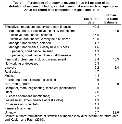
[SOURCE: Jobs and Income Growth of Top Earners and the Causes of Changing Income Inequality: Evidence from U.S. Tax Return Data,34]

Trends in the Top One Percent

We know from the analysis of inequality trends at the beginning of this series that the one percent has increased its share of total income in the US over time, but here is a helpful reminder of that trend, with updates through 2013:

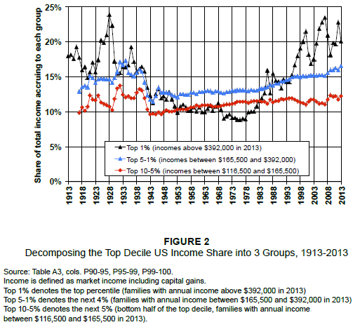
[SOURCE: Striking it Richer: The Evolution of Top Incomes in the United States by Emmanuel Saez, 8]

It is clear from these trends that the top one percent has played a huge part in the increase in inequality in the United States since the 1980s, and that the longer-term trend has not changed even while the recessions have caused some volatility in top shares. Emmanuel Saez, in Striking it Richer: The Evolution of Top Incomes in the United States,  points out the stark inequality of growth since the great recession:

“From 2009 to 2012, average real income per family grew modestly by 6.9% (Table 1). However, the gains were very uneven. Top 1% incomes grew by 34.7% while bottom 99% incomes grew only by 0.8% from 2009 to 2012. Hence, the top 1% captured 91% of the income gains in the first three years of the recovery.” 1

Whether this trend will continue depends on a number of factors, including the causes of the increases and future policy decisions related to economic growth, regulation and redistribution.

Explanations of Gains in the Top One Percent

There are four major explanations used to explain the increasing share of income absorbed by the top one percent. These include: Globalization, Skill-Biased Technology, Superstar theory, and Compensation Norms. I will review each one briefly here.

Globalization

The globalization theory argues that the opening of borders and increasing global connectedness has increased demand for high-skilled jobs in the United States and decreased demand for low-skilled jobs, relative to demand abroad. This fits with the trend within the top one percent, in that increased labor compensation is an increasing proportion of total income. However, it does not fit a simple supply and demand framework when considering that other high income countries have not seen the same relative increases in income. For example, Saez, Piketty, Atkinson and Alvaredo in The Top One Percent in International and Historical Perspective, make the following observation:

“While other English speaking countries have also experienced sharp increases in the top 1 percent income share, many high income countries such as Japan, France, or Germany have seen much less increase in top income shares. Hence, the explanation cannot rely solely on forces common to advanced countries, such as the impact of new technologies and globalization on the supply and demand for skills.”

Skill-Biased Technology

We have reviewed this theory before, which argues that technology can act as a complement to some jobs and a substitute for others. For this theory to fit with the increase in the top one percent’s increase, it would imply that technology acts as a complement for high-skilled, high-income executive and finance jobs while acting as a substitute for lower-skilled jobs, thus increasing the compensation and share of total income going to the top one percent.

Superstars

The “superstar” explanation is a play off of the previous two theories, arguing that globalization and technology (especially communications technology) have created a situation that allows high-performing individuals to expand the scale and reach of their market base. This is most easily imagined for performing artists who are typically referred to as superstars, like singers and actors, but can also be used to explain the increases in other occupations as well.  (Kaplan and Rauh, 43)

Compensation Norms

The next theory is a bit more involved, so I will spend more time on this. The compensation norms theory argues that social norms regarding increased CEO compensation have shifted to permit higher inequality within a company, and similarly argues that some of the gains at the top are due to rent-seeking behavior and information asymmetry.

 

Changes in pay norms:

Pay for performance and merit-based pay schemes became more common in the 80s and 90s, at the same time unionization declined. This shift away from job-based pay schedules toward merit-based fits the narrative that top compensation is partially a result of changing social norms. (Saez et. al., 11)

It is also evident that most of the increased share going to the top is a result of increased pay for executives and financial professionals. According to Bakija, Cole and Heim, “Executives, managers, supervisors, and financial professionals… can account for 70 percent of the increase in the share of national income going to the top 0.1 percent of the income distribution between 1979 and 2005.” (2) That divergence could be evidence that compensation norms for some occupations have changed while others have not. It may also be evidence of market inefficiency or rent-seeking behavior.

However, Kaplan and Rauh point out that the theory of changing social norms does not hold up when considering that CEOs of public corporations who are subject to peer review of compensation, have seen their pay increase by less than the pay for CEOs of private corporations whose compensation is undisclosed. By contrast we would expect the compensation to increase at similar rates if social norms related to CEO compensation were more generous. (Kaplan, Rauh, 39)

 

Rent-Seeking Behavior

Finally, another explanation related to compensation norms is that of rent-seeking behavior. Rent-seeking describes activities or behaviors used to increase compensation beyond a level considered market-efficient. Typically, rent-seeking behavior includes lobbying for corporate subsidies or tax incentives, but it can happen for other reasons as well, including information asymmetry or compensation spillover effects.

Bakija, Cole and Heim review the diversity of income concentration going to different occupations in the top one percent, and find considerable heterogeneity, graphed below. In particular they find that financial and real estate professionals saw the highest growth. (Page 23-4) Considering anecdotally that these increases occurred largely during the housing bubble, a period of significant deregulation of the real estate and financial sector, one could argue that this growth is not reflective of an efficient market distribution of income.

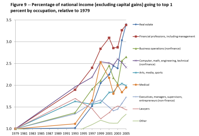
[SOURCE: Jobs and Income Growth of Top Earners and the Causes of Changing Income Inequality: Evidence from U.S. Tax Return Data by Bakija, Cole and Heim]

Other evidence of rents proposed by Josh Bivens and Lawrence Mishel, in The Pay of Corporate Executive and Financial Professionals as Evidence of Rents in Top 1 Percent Incomes, include the stark difference in CEO compensation across the globe:

“A survey by Towers Perrin, a consulting firm, shows U.S. CEO compensation was triple that of other advanced nations in 2003, up from 2.1 times foreign CEO compensation in 1988 (Mishel et al. 2004, Table 2.47). Tower Perrin also reports that U.S. CEO compensation was 44 times that of the average worker whereas the non-U.S. ratio was 19.9.” 8

Similarly, they remind readers that occupations in the financial sector (think Wall Street jobs) often have the opportunity to shift rents to themselves, particularly in situations where there is significant information asymmetry and high-risk poorly-understood financial products like CDOs on the market. (Bivens, Mishel, 9)

If they exist, these rents represent inefficiencies in the market that can be reduced without harming overall economic growth. In other words, marginal tax increases on high incomes to reduce the existence of rents would work to redistribute labor income without harming the economy. However, if the increased compensation is not a result of rents but rather market-efficient responses to increasing scale (superstar), globalization or skill-biased technologies, then tax increases may result in some adverse affect to overall economic growth.

---

Understanding the increase at the top of the income scale is challenging. There are a number of factors, including many unseen, making it nearly impossible to establish consensus among researchers. And of course, policy solutions will be as diverse as the explanations they accompany.

Beginning next week we will shift our focus to intergenerational mobility, looking particularly at how children of each bracket move into other (higher or lower) income brackets as adults. As always, you can contact me through my Contact Page, and find the reading list here, with updated dates: inequality-social-mobility-and-public-policy-syllabus

 

Persistent Poverty

This week we will be focusing on explanations of persistent poverty.

What is “persistent” poverty?

The description of persistent poverty is used to distinguish long-term poverty spells from those that are more transient in nature. In fact, most Americans will experience a poverty spell in their lifetime, so it is important to understand the difference between a relatively short incidence of poverty, due to job loss, sickness or some other life incident that results in a short term loss of income compared to a longer-term incidence of poverty that is not as easily recoverable. That being said, poverty can also be described as chronic or long-term within an individual’s life and not necessarily be “persistent” if their children grow up to earn a higher income as adults. Generally when people talk about the “persistently poor” they imagine poverty that persists from generation to generation. Of course, chronic and persistent poverty are related when the chronic poverty of a parent leads to lower outcomes for their children.

Persistent poverty is one primary concern of those who study inequality. The fear is that high inequality may in effect cause persistent poverty if class stratification becomes so divergent that it becomes extraordinarily difficult to enter from the “underclass” to the “upperclass.” Whether inequality causes this type of immobility will be explored later as we get into studies of intergenerational mobility.

Who experiences persistent poverty?

Policy discussions of ending poverty often focus on poor children, who can hardly be blamed for being born into a situation that places them at a significant disadvantage. In the long-term Panel Study of Income Dynamics (PSID), just under 10% of children had family incomes below the official poverty line for more than half of the period between 1979 and 1994. (The Economic Costs of Poverty in the United States: Subsequent Effects of Children Growing Up Poor, 12)

A study by Mark Rank and Thomas Hirschel of The Likelihood of Poverty across the American Adult Life Span found that by age 65 more than half of adult Americans will have experienced at least a year of poverty, and that most spells last for only a few years. They also found that the probability and average length of poverty is significantly different by race:

“One quarter of white Americans experienced poverty at some point during the 13-year [study] period compared with two-thirds of black Americans. Furthermore, 67 percent of white Americans who experienced poverty were poor for three years or less, whereas the figure for black Americans was only 30 percent. Consequently, black Americans were more likely to be touched by poverty and more likely to be exposed to poverty for substantially longer periods” (Rank, Hirschel 202)

Even more striking, they found that by age 75, Black Americans had over a 90% chance of experiencing poverty, while for White Americans that probability was just over 50%. This extreme gap can be seen clearly in the graph below.

[IMAGE SOURCE: Rank and Hirschl, 211]

Unsurprisingly, another study by a researcher at the Census Bureau found that people who experience chronic poverty (defined in her study as people who experienced one or two spells of poverty totalling 90% of a four year period) are more likely to be “Black, Hispanic, under the age of 18 or over the age of 65, and without a college education.” They are also more likely to be female and live with a female head of household. In addition, approximately one third had a disability that limited work. (Edwards, 9)

Geography also plays a role in persistent poverty. The Economic Research Service at the US Department of Agriculture defines persistent poverty at the county level, with those counties who have 20% or higher poverty for 30 years as persistent poverty counties. The vast majority of these 353 counties are located in the south and 85% are nonmetro areas, as you can see on this map:

[IMAGE SOURCE: USDA, Economic Research Service]

Why does poverty persist?

This question is really the heart of the matter, because any effort to reduce poverty or its persistence requires answering “why” first. There are a number of theories posited to explain poverty, and recent research on neighborhoods and child brain development has added significantly to the knowledge base. Here I will outline a few of the major theories.

Cultural Explanations

Cultural explanations are popular for explaining poverty because people who are poor seem to operate differently than people who are not poor. While of course the experience of poverty will affect people’s behavior, this explanation sometimes stems from harmful stereotypes that poor people are lazy, entitled, and morally bankrupt.

In “Culture” and the Intergenerational Transmission of Poverty: The Prevention Paradox, Ludwig and Mayer explore the notion that a traditional family structure, parental work and religion could reduce poverty, an idea sometimes perpetuated by policymakers. They first remind readers than many adults who experience poverty were actually raised in this “ideal” type of situation that policymakers promote as the cure to poverty and emphasize the limitations of cultural change as policy. Then, even accepting this as truth, they find that “If eighth graders lived with their biological parents, at least one parent worked, and the child attended religious services, poverty in their generation would fall by 22 percent, assuming that the effects of these indicators of culture on children’s poverty status are entirely causal.” (187) Hardly a silver bullet.

There is merit however in explanations that revolve around the concept of social exclusion and networking gaps. In Understanding Persistent Poverty: Social Class Context in Rural Communities, Sociologist Cynthia Duncan explains how class cultural divides can cause challenges when people who grew up poor try entering the working world. She emphasizes research by others that demonstrate how “participation requires talking, thinking, and acting like those who manage America’s institutions,” and how when poor people do not have the same cultural ‘toolkit’ as those who grew up nonpoor, they find it more difficult to enter mainstream society and network for opportunities. (108)

Political Economy or Institutional Explanations

Institutional explanations are often seen as the opposite of cultural explanations, because while the impetus for change under cultural theories rests largely on the poor themselves, the impetus for change under institutional explanations rests on the state. Institutional explanations do not mean easy solutions however, as they include the likes of institutional racism and historical and political power differentials. Considering the racial and geographic dynamics described above, historical explanations are more than appropriate to consider.

Cynthia Duncan did research in rural Texas, Mississippi and Appalachia and illustrates in her paper how the political economy of these communities is structured in a way that maintains stratification:

“Accounts of rural life in the deep South describe rigidly stratified communities. The poor are completely dependent on the wealthy, who maintain their privilege through control over labor and most social institutions that affect the poor… Given this social structure, the poor have no opportunities to improve their status, and their limited prospects engender a kind of fatalism that eschews achievement and individual mobility. The ‘cultural tool kits’ they develop do not equip them for mobility, and everyday interaction reminds them of their place at the bottom.” (Understanding Persistent Poverty: Social Class Context in Rural Communities, 112)

Neighborhood or “Place” Explanations

Institutional and historical explanations also tie in with neighborhood explanations that have become more dominant recently thanks to work by Harvard economist Raj Chetty. (If you are interested, you can watch a recording of a presentation by him at a Center on Budget and Policy Priorities event here: The Role of Neighborhoods in Persistent Poverty).

The idea is that the place in which one grows up has a significant impact on future potential. Presumably, areas with higher densities of poverty have less social capital and opportunities than areas with lower poverty.

An experiment called Moving to Opportunity in the US studied the effect of neighborhoods by moving poor people out of high poverty neighborhoods and into low poverty neighborhoods using randomized housing vouchers. It was only fairly recently that the longer term impacts of the study were evaluated by Chetty and others, who found that those who moved to a low poverty area before 13 years of age earned on average $3,477 more per year in their mid-twenties compared to those who did not. (The Effects of Exposure to Better Neighborhoods on Children: New Evidence from the Moving to Opportunity Experiment, 1)

“We estimate that moving a child out of public housing to a low-poverty area when young (at age 8 on average) using an MTO-type experimental voucher will increase the child’s total lifetime earnings by about $302,000.” (Chetty et al, 5)

In Understanding Persistent Poverty: Social Class Context in Rural Communities, Cynthia Duncan describes how a community with a large middle class may be less stratified and so more inclusive, with better opportunities for networking and increased social capital. However, the MTO experiment found negative effects on those who moved after the age of 13 and no effect on the adults who moved. This indicates that neighborhood has significant effects on development, which brings us to the final explanation.

Developmental Explanations

How poverty affects the brain has been a sensitive research subject for many years and is conducted delicately so as not to cause policymakers to get the wrong idea about the correlation between poverty and cognition. However, there is new evidence to suggest that poverty has a significant impact on brain development in early childhood, especially among children under 5 years of age. (The Long Reach of Early Childhood Poverty, 25).

In The Long Reach of Early Childhood Poverty, Greg Duncan and Katherine Magnuson outline the long term effects of child poverty, including the completion of schooling, income and work hours, while also highlighting that poverty during adolescence may also have future effects on health and birth outside of marriage. To illustrate these effects, the authors presented the following charts:

[SOURCE: Duncan and Magnuson, 27]

Looking Forward

Recent research has led to some major breakthroughs, especially about the importance of targeting poverty assistance at young children. The Moving to Opportunity experiment has demonstrated positive neighborhood effects on young children while scientists have discovered a link between brain development and poverty that has similar implications.

The persistence of poverty is an issue that we will continue to explore from the angle of intergenerational mobility. Knowing that many Americans experience poverty firsthand is important when considering downward mobility, while understanding some of the causes of intergenerational and persistent poverty will help explain some of the immobility at the bottom.

Next week we will explore the top one percent as a contrast to the description of persistent poverty, before we begin a four week segment on intergenerational mobility.

As always, you can leave me a message through the Contact Me page, and you can find the reading list here:inequality-social-mobility-and-public-policy-readings-schedule

Inequality: Deunionization

“From 1973 to 2007, private sector union membership in the United States declined from 34 to 8 percent for men and from 16 to 6 percent for women. During this period, inequality in hourly wages increased by over 40 percent.” (Western and Rosenfield, Unions, Norms, and the Rise in U.S. Wage Inequality, 513)

This week we focus on the impact of deunionization on wage inequality, complementing the trends in skill premiums and job polarization described last week. 

Unions increase wages. That much is clear from the literature, with the union wage impact estimated to range between 10-20%. However, the impact is not the same everywhere, for everyone, in every industry. So before we begin analyzing the impact of deunionization on wage inequality, I thought I would lay out what researchers have found about the union effect:

1. The union effect generally falls during periods of inflation and increases during recessions.
2. Unionization raises wages the most for young people and those with little tenure.
3. Unionization has a much bigger impact on blue collar jobs (19%) than white collar (4%).
4. The union impact varies based on the size of the company and the percent unionized, with smaller companies and greater proportions increasing the union effect.

(Freeman, Medoff Chapter 3)

Spillover Effects

Unions are generally a force for equality both in the workplace and larger community. In addition to quantitative analyses of the union impact, researchers describe something of a “moral economy” that is promoted by unions, which spills over into the economy by changing norms and expectations of wage equity. (Western, Rosenfield 514)

For example, companies regularly use wage surveys to estimate competition in the region and adjust accordingly, raising wages for non-unionized firms in proximity to unionized firms.  Freeman and Medoff also find that  approximately 20% of unionized firms pay their non-union employees in line with union agreements, and that workplace rules tend to spill over, evidenced by the erosion of merit pay and emphasis on seniority in layoff decisions. Finally, they found that within companies where blue-collar workers are unionized, white-collar employees benefit from improvements in fringe benefits, though their wages are seemingly unaffected (Freeman, Medoff Chapter 10)

Impact on Inequality

Researchers have long been concerned that social benefits of the union effect are offset by increased unemployment and depressed wages among non-unionized employees, resulting in a net increase in inequality by creating a gap between covered and non-covered employees.

Richard Freeman and James L Medoff consider this at length in the book “What Do Unions Do?” and discover that although unions do raise wages at the expense of others, there are three other benefits that offset it in favor of reducing inequality:

“…the increase in inequality induced by monopoly wage effects is dwarfed by three other trade union effects on wages that reduce inequality: union wage policies lower inequality of wages within establishments; union wage policies favor equal pay for equal work across establishments; and union wage gains for blue-collar labor reduce inequality between white-collar and blue-collar workers.” (Freeman, Medoff 78)

Freeman and Medoff’s book was published in 1984, so while it provides a good description of the benefits of unionization, it predates much of the significant decline in union membership described in the opening quote.

According to Nicole Fortin and Thomas Lemieux in Institutional Changes and Rising Wage Inequality: Is There a Linkage?, unionization declined slowly in the 60s and 70s and fell especially fast in the 80s (at the same time wage inequality increased) before slowing again in the 90s. (77) They found that deunionization has had a significant impact on wage inequality for men, but not women.  This is because unionization had a stronger equalizing effect for men, while most women who were unionized were relatively skilled, tempering the equalizing effect. (80)

The equalizing effect of unions can be seen in the following graphs, where the distribution of union wages are more concentrated around the average while nonunion wages are more spread out across the range. It is also clear when moving from 1979 to 1988, that as the proportion of union wages decreases, the overall spread in wages increases (though for women the minimum wage has a clearly more dominant role):

[Source:  Institutional Changes and Rising Wage Inequality: Is There a Linkage?, 85]

Fortin and Lemiuex conclude that deunionization had no effect on women but that for men, “the variance in log wages would have increased by 21.3 percent less if the rate of unionization had remained at its 1979 level.” (89)

In contrast, In Unions, Norms, and the Rise in U.S. Wage Inequality, Western and Rosenfield expanded the analysis of deunionization on inequality to include the spillover effect of unions on nonunion wages. After adjusting for these spillover effects, they conclude that deunionization can explain 20% of the increase in inequality among women and 33% for men.

Western and Rosenfield also find that most of the increase in inequality in the 90s stems from increases in “within-group” inequality. In other words, the variance of wages within groups of individuals with similar characteristics increased over this time period more than the variance of wages between groups of individuals with different characteristics. Similarly, they find that deunionization impacted mostly within-group inequality.

Impact on Working Poverty

Having established a link between deunionization and increased wage inequality, David Brady, Regina S. Baker and Ryan Finnigan explore the impact of deunionization on working poverty in When Unionization Disappears: State-Level Unionization and Working Poverty in the United States. Working poverty is a description used for officially poor households who have at least one worker (10.4% of families in 2004). (873) While the authors recognize that most union workers are earning above median wages and thus that most working poor are not unionized, they determine that the spillover effects have an impact on low wage workers in a way that does impact working poverty.

The broad relationship between unionization and working poverty can be seen in the following graph. States that have higher rates of unionization have fewer working poor as a percent of their population compared to states with low rates of unionization.

[Source: When Unionization Disappears: State-Level Unionization and Working Poverty in the United States,880]

Using a two-way fixed effect logit model of working poverty, the authors find that increases in state-level unionization decreases working poverty significantly, outweighing even the economic performance or social policies of the state. More specifically they find that “for a standard deviation increase in state-level unionization, relative working poverty in non-union households is expected to decline by a factor of 1.3” (888)

The authors also find that at the individual household level, the characteristics of education, part-time employment and having multiple earners still remain the most important predictors of poverty. However, state-level unionization arguably rival other individual-level characteristics including race or being a single mother. (885) This result has significant implications for future poverty research.

Looking Forward

There is some concern that unions have lost their bite as membership has declined. In Economic Impacts of New Unionization on Private Sector Employers: 1984-2001, John DiNardo and David S. Lee use a regression discontinuity approach to compare manufacturing plant wages that became unionized after barely winning an election to manufacturing plant wages where unions barely lost. Among these newly created unions, they found no statistically significant difference in wages, concluding that new unions have not been successful at increasing average wages. (DiNardo,Lee 1431)

The research described herein indicate that unionization, especially when incorporating spillover effects, may explain some of the increase in wage inequality over the 80s and 90s. It also may help explain differing rates of working poverty in the US. How this research will fit into policy decisions in the future is yet to be seen.

Next week we will be shifting our focus a bit. While the first four weeks have been focused on trends in inequality, we will be focusing on persistent poverty next week, followed by a focus on the top one percent. At that point we will shift into an analysis of intergenerational mobility.

As always, feel free to send me a message through the contact page. The reading list for each week can be found here: inequality-social-mobility-and-public-policy-readings-schedule

Inequality: Wages

“What primarily characterizes the United States at the moment is a record level of inequality of income from labor (probably higher than in any other society at any time in the past, anywhere in the world, including societies in which skill disparities were extremely large).” Piketty 2014, 265

This week we explore explanations for wage income inequality in the United States. Next week we will explore the role of deunionization in more detail. 

So far we have discussed inequality with a clear underlying assumption that inequality is bad, and equality is good. But this is not exactly the case, and in fact there is significant value to inequality as an incentive to work hard, build new skills, and increase educational attainment. In the United States especially, where higher education is often financed, education would be a net drain on lifetime wealth in the absence of inequality, or the expectation that education will pay off in the long run.

The real worry then, is two-fold: first that individuals at the bottom are struggling, which causes a number of problems for society including increased crime, and second that mobility up and down the economic ladder slows down or halts because those born in families at the bottom of the ladder can’t afford to or do not have the necessary knowledge to invest in skills and education, and those born in families at the top are significantly and perhaps unfairly advantaged (family income and parent educational attainment being the biggest predictive factors in a child’s future).

We already know from week one that income inequality in the United States has increased over the last 30 years, to the point that Piketty made the bold claim (quoted at the beginning of this post) in his book, Capital in the 21st Century. But what are the reasons behind this increase? And what are the implications?

A number of mechanisms have been suggested by economists, and I use the word suggested because it is notoriously difficult to establish causal relationships in public policy issues this large, especially when dealing with limited data. Usually the best we can do is explore trends, establish correlations and theorize based on the picture we find. Some of the main theories include:

Increased Education/Skill Premium

One explanation of increased wage inequality is that the premium for high-skilled jobs has increased relative to low-skilled jobs. In other words, the value that the market places on jobs that require higher education has increased over time at the same time the value that the market places on jobs that require no education has decreased, slowly but surely widening the gap.

There is evidence of this phenomenon. The earnings gap between those with a high school education and those with a college education has increased considerably over the past thirty plus years. In dollar terms, the earnings gap in 1979 was $17,411 between the median high school educated and college-educated individual. In 2012, it was twice that at $34, 969. (Autor, 844) This trend has been worse for men than women, with male high school dropouts seeing mostly negative changes in real wage levels since 1990:

[Source: Skills, Education and the Rise of Earnings Inequality among the “other 99 percent”, 849)

This wage premium seems to explain about 50-70 percent of the increase in wage inequality over this time period, based on a number of studies. The most robust explanation for the wage premium has to do with supply and demand, which we explored a bit last week. (Autor)

A subset of this theory involves the concept of “hypermeritocracy” and the rise of supersalaries. The examination above does not explain the extreme increase in salaries among the top 1%, but it is worth mentioning because the top percentile has collected over 10% of total US labor income since the late 90s (but only 5% in 1970):

[Source: Capital in the 21st Century, 292]

It is also worth mentioning because although many place their focus on the extreme incomes of superstars like actors and NFL players, most of these increases can be traced back to the very high salaries for managers and top executives (who make up about two-thirds of individuals in top 0.1 percent).  (Piketty 264-66, 298-303)

Lifecycle trends

Another explanation of wage inequality is that of lifecycle trends. The lifecycle theory of inequality makes a lot of sense, and provides another reminder that inequality is not necessarily a bad thing. As a natural and desired part of a lifecyle, income increases as an individual enters the working world, moves up, earns raises, saves, and then declines as the individual enters retirement and begins living off savings.

While this does explain some of the baseline inequality, it does not do a good job of explaining the increase in inequality, and in fact there is evidence that “the concentration of wealth is actually nearly as great within each age cohort as it is for the population as a whole,” which essentially eliminates lifecycle trends as a causal mechanism (Piketty, 244). In addition, for the lifecycle trend to explain increased inequality it would also mean that an individual was highly mobile: moving into jobs with significantly higher skill and pay levels at their peak. And this simply isn’t the case for the vast majority of workers. (Piketty, 299)

Job polarization

The job polarization theory boils down to this:

“The structure of job opportunities in the United States has sharply polarized over the past two decades, with expanding job opportunities in both high skill, high wage occupations and low skill, low-wage occupations, coupled with contracting opportunities in middle-wage, middle-skill white-collar and blue-collar jobs.”
(The Polarization of Job Opportunities in the U.S. Labor Market, Autor 1)

If true, the relative polarization of job opportunities, combined with the increase in the education/skill wage premium and the reduction in real value of the minimum wage, would explain the increase in wage inequality. Job polarization can be seen in the following chart, where ‘middle skilled’ jobs, classified here as office and administrative jobs, production and craft, and operators/laborers, have seen reduced employment since 1979, while jobs in high and low skilled jobs have seen increases in employment:

[Source: The Polarization of Job Opportunities in the U.S. Labor Market, Autor 8]

Interestingly, there are significant differences by gender. Decreases among men in middle skilled positions shifted relatively equally to high and low skilled positions, whereas women shifted largely to higher-skilled positions. [This is partly a result of education trends]:

[Source: The Polarization of Job Opportunities in the U.S. Labor Market, Autor 9]

Some of these occupation shifts can be explained by increases in the proportion of Americans with higher education generally, especially among women. Other explanations include technology substitution of routine-task jobs and the relative increase in demand of high-skilled jobs that use skill-biased technology as discussed last week. (Autor)

Another explanation that is frequently cited, and rose to the fore last election cycle, is the hollowing out of middle-income jobs due to increased international trade and offshoring. However, Piketty makes the point that this is not a very robust explanation. In fact, “the United States’ internal imbalances are four times larger than its global [trade] imbalances. This suggests that the place to look for the solutions of certain problems may be more within the United States than in China or other Countries.” (Piketty 297-8) That said, for a subset of individuals who were directly affect by trade, this explanation holds significant weight. It is also important to consider the fact that offshoring and trade has been largely made possible by improvements in technology.

The job polarization theory is convincing, but as with all theories there are critics. In Assessing the Job Polarization Explanation of Growing Wage Inequality, authors Mishel, Schmitt and Shierholz point out that the contraction of middle income jobs has a trend that begins prior to the increase in wage inequality, which eliminates the possibility of a cause-effect mechanism. They also point out occupational explanations do little to explain wage trends in the 2000s, and generally dismiss it as too narrow of an explanation that does not include the full picture.

Devalued Minimum Wage and Deunionization

In addition to the explanations above, generally noted in these studies is the reduced value of minimum wage and deunionization, but as I will be exploring those in more depth later, for now just know that they are considered to play into these trends, at least for the middle and lower end of the skill/income range.

Clearly this is a complicated issue that must take a wide scope of analysis to unravel, but it is helpful to know some of the mechanisms behind these changes in order to develop effective policy solutions. There is plenty of room for future research.

Next week we will explore the role of unions in the US and how they may or may not explain trends in inequality. The reading list can be found here: inequality-social-mobility-and-public-policy-readings-schedule.

As always, feel free to leave comments or send a message through the Contact page.

 

Inequality: Technology and Capital

This post reviews the role of capital accumulation in inequality and how technology, as both a substitute and supplement to labor, has had a noteworthy effect on wage trends and inequality. 

Thomas Piketty’s book, Capital in the Twenty-First Century, brought rising inequality to the attention of the media and policymakers and contributed much to the discussion, in addition to drawing a lot of criticism. His book discusses the increasing role of capital in inequality and warns that it will only get worse without significant intervention.

Piketty defines capital as “the sum total of nonhuman assets that can be owned and exchanged on some market.”(48) This excludes human capital but includes what he calls “immaterial” capital, or what I would call identifiable intangibles, including assets like patents and the value of brand and reputation that is wrapped up in stock prices. (49)

Piketty makes a number of points about trends in capital including the following:

1. The makeup of capital over the long term has shifted largely from being land-based in the eighteenth century, to now mostly financial and industrial capital. (42)
2. While capital can be owned publicly or privately, most capital is private. (46)
3. Globalization has increased cross-country ownership, such that many countries earn income from capital located in other countries. However, this point shouldn’t be too alarming because most countries end up having a national income within 1% of domestic output. (44)
   1. Note: This is not to say that global inequality does not exist. On the contrary, domestic output and per capita GDP is highly unequal, though it has been converging since the mid twentieth century. (60) Moreover, “the global income distribution is more unequal than the output distribution, because the countries with the highest per capita output are also more likely to own part of the capital of other countries with a lower level of per capita output.” (67-68)

The first chapter of his book is most important because it is where he lays out “The First Fundamental Law of Capitalism” which forms the basis for his main argument (52). He explains here that capital’s share of national income (as measured annually) is a function of the capital/income ratio (national capital stock divided by national income) times the rate of return on capital.

α = r x β

Where:
α = capital’s share of national income
r = the rate of return on capital
β = the capital/income ratio (52)

This relationship matters for inequality because, holding all else equal, as the capital/income ratio increases (as trends suggest will occur), capital’s share of national income increases. And because capital income is a greater share of individual income at the top, that accumulation of wealth increases inequality. Piketty’s major premise in his book is that inequality will increase as long as the rate of return on capital is greater than the rate of income growth: r > g. This assumption that the rate of return on capital will exceed growth for a sustained period of time is the main point of contention among critics. For one exploration, see Is Piketty’s “Second Law of Capitalism” Fundamental?.

In After Piketty?, economist A.B. Atkinson responds to Piketty’s book by considering a number of policies that might work to reduce inequality. I will only highlight two here, but he emphasizes that responses to rising inequality should come from many policy areas, not just those related to tax and spending.

“Inequality is as much a matter for the Minister responsible for science as for the Minister responsible for social protection.” (620) 

Atkinson discusses in part how technology can act as both a substitute for labor and a supplement to labor. He explains that as capital increases relative to labor, wages rise and the rate of return on capital decreases. But eventually, capital (technology) can reach a point of substitution, whereby capital income increases but labor does not benefit. And as discussed above, that impacts inequality because capital income is concentrated at the top, while middle-income folks depend primarily on wage income.

Atkinson argues however that the role of technology is not out of our control, and that investments in technology that increase the productivity of workers could be encouraged by government to balance investments in technology that act to replace labor. At the same time, he argues that bargaining power between capital and labor need also improve, a topic that we will be covering in two weeks.

Unlike Atkinson, in Separating Efficiency and Equality, Automation and Piketty’s Theory of Increasing Capital Share, Yew-Kwang Ng argues for more general tax and spend policies rather than issue specific policies. He also tempers the argument that increased technology will exacerbate inequality. He reminds us that there was a great fear of mass unemployment in the 1970s due to the rise of the personal computer, a fear that was not realized. He argues that to the extent technology complements labor and raises output, it increases the demand for labor, preventing massive unemployment. The problem, he conjectures, will be more with a lack of skilled labor than a lack of jobs.

Which brings us to the next reading on the list, The Race Between Education and Technology. [Full disclosure: I couldn’t access the book in time for this blog so I settled with reading this 2007 working paper version].  The paper discusses how the relative supply of educated individuals serves to affect the wage premium of education, and at the same time how technology is skill-biased.

“The two most important forces in the framework concern the change in the relative supply of more-educated workers, which has mainly occurred through changes in schooling, and the changes in the relative demand of more-educated workers, which has been driven by skill-biased technological change.” (6)

The authors explain that in the late twentieth century much of the increase in wage inequality can be explained by the increase in the education wage premium (an increase of 23% between 1980 and 2005), but that this was mainly a result of slower growth in the supply of college workers since 1980. At the same time, technology advances tend to be skill-biased, such that they increase the relative demand for more skilled workers over the unskilled. In other words, demand for skilled workers exceeded its supply over this time period, increasing the wage premium of education and subsequent inequality. “The race had been lost to technology.” (28)

So, what do we know?

1. The relative growth of capital in a country, and the rate of return to that capital, matter when considering inequality. This is because capital income is a greater share of individual income at the top.
2. There is a great deal of criticism around Piketty’s assertion that r > g .
3. Technology can act as a substitute and supplement to labor. How technology impacts capital income inequality will depend on the elasticity of substitution and how technology serves to complement labor.
4. The way in which technology impacts wage inequality depends not only on the substitution/supplement aspect, but also on the relative supply of skilled labor for skill-biased technology.
5. In general, the main takeaway for me is that capital accumulation, increases in technology, and the relative skilled labor supply all serve to affect vertical inequality, as those who are more privileged (educated, skilled, capital income-earning) reap most of the benefits of these trends, while those less privileged will be left behind without intervention by policymakers.

Next week, we will be focusing specifically on wage inequality. The associated readings can be found linked to my first blog post.